Basic Concepts
Consider yourself a simple organism. You have two main concerns in life (whether you realize it or not): to survive and to reproduce. Your survival depends upon how well you cope with the environmental challenges that come your way. Change of any kind presents a challenge. Are you genetically predisposed to overcome specific problems that come your way, or does your genetic makeup let you learn from a situation and adapt quickly (in that, before you die and, therefore, cannot reproduce)?
It is this adaptation and survival of the fittest that is of particular interest in problem solving. In a population, there will be individuals that cannot adapt to potentially life-threatening problems that may arise and will be eliminated from the gene pool. Others will be better suited to overcoming or solving those problems and will have a better chance of passing their genes (or parts of them) along to offspring.
This scheme can be considered in the light of general problem solving. There is a set of solutions (the population and their characteristics and abilities) for a given problem or set of problems (surviving in a given environment or facing a specific change or challenge). A fitness test (those who survive) determines the viability of the solutions (which individuals in the population are allowed to reproduce).
Some biology terminology needs to be considered at this point. A "gene" represents some trait of an individual (for instance, the color of one's hair). How that trait is expressed or, in other words, the possible values or versions of that trait (for one's hair color, this might be black, brown, red, blonde, and so on) are called "alleles." A group of genes is called a "chromosome." The specific position in a chromosome on which a gene is located is referred to as its "locus." The collection of chromosomes that make up an individual is called that individual's "genome." "Haploid" and "diploid" refer to individuals with unpaired and paired chromosomes, respectively.
In a problem-solving realm, you can consider that the traits expressed by each individual's genes either help or hinder it in its ability to resolve the challenges with which it is faced. How can this scheme be applied to "artificial" systems and the problems that they are trying to resolve?
Application Example
Much of my current work has involved in-circuit emulator software. An in-circuit emulator (ICE) is a hardware debugging tool that, through its own on-board, modified processor, lets you emulate a like processor or family of processors on a target system. Through this special on-board processor, along with additional hardware and memory, you can direct and monitor code execution, examine memories, and so forth, providing a window into your code and its operation.
One of the features of an ICE is the ability to provide a program (internal) clock, essentially the heartbeat of the hardware being designed and tested. On the particular ICE unit for which I am writing software, users can enter a value from 32 KHz to 40 MHz for the clock speed. The ICE hardware uses a Cypress CY22393 programmable, multiple-clock generator chip. One of the clock outputs on this device is set up in order to provide the program clock. The setting-up of the clock is the operation that lends itself to a genetic algorithm.
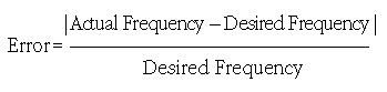
The clock chip uses a reference clock and four values programmed into it to arrive at a desired output frequency. These values deal with the feedback loop of the phase locked loop and dividers that are applied to it. Figure 1 shows this formula.
The reference clock or frequency is fixed, but the other values have specific ranges over which they may vary (Table 1). Given the four variables and their ranges, there are some 66,584,576 programmable combinations. These combinations will produce not only a wide range of frequencies but also duplicates of those frequencies.
On a 450-MHz Intel Pentium III system, examining each combination took approximately 20 seconds. For most users, this would be too long a time to wait for determining the proper value combination for the desired frequency, especially if they were changing frequencies often during the testing of their target system.
I've determined that a frequency error or deviation of not more than 0.02 percent is acceptable, with a deviation of not more than 0.01 percent being preferred. This means, for example, that for a desired frequency of 16.5 MHz (16,500,000), an actual frequency ranging from 16,496,700 to 16,503,300 would be acceptable within my company's specification (this is some 200 parts per million deviation). Obviously, the closer the actual frequency is to the desired frequency the better. I believed that using a genetic algorithm to obtain the device values would, in most instances, produce short calculation times, and that the process would also provide the necessary accuracy.
I'll now examine how you represent this problem in terms of genetic algorithms and how genetic adaptation can be used in arriving at a targeted solution from a population of general solutions.
The first step in gene representation is to define a population of individuals that provide the information necessary to supply input into the formula described previously. It is important to note that I have defined what the problem is (finding an accurate, desired output frequency given a specific formula and input ranges to that formula), but not how the problem is to be solved (how the optimum inputs are to be arrived at).
This problem must now be encapsulated into artificial genes and chromosomes. The formula has four main components that can vary: P, PO, Q, and Divider. These values can be defined as bit fields in a simple 32-bit program variable. Figure 2 shows how these will be placed in a 32-bit variable.
Each segment of this variable, which represents one of these components, can be viewed as a gene. Grouped together, they can be viewed as a chromosome. Each individual in the population will have only one of these chromosomes (a haploid individual).
I start off the operation with a population of 500 individuals whose gene values are randomly generated. Table 2 shows a sampling of 20 individuals (4 percent) taken from this initial population. As can be seen, their chromosome values are varied as are the resultant frequencies based on those chromosomes. This variation is crucial to finding a proper solution over time as it provides a large solution base from which offspring that solve a specific problem (namely, finding the proper program values for a given frequency) may be produced.
One of the most important aspects of a genetic algorithm is the selection of a proper fitness function. This is the criterion by which the individuals in a population will be determined fit enough to be selected for reproduction. A poor fitness function will result in a generation of offspring that may be no closer to solving the problem than their parents. Indeed, poor selection may result in offspring that are even worse at solving the problem. A poor fitness function may likewise result in populations of offspring that get stuck at inappropriate maximum or minimum locations in the solution set from which they cannot escape.
My goal again is to arrive at device program values that will produce the closest actual frequency to a desired frequency in the shortest amount of time. How do I measure the success of each individual in the population in approaching this goal?
Again, the company goal is an error factor of no more than 0.02 percent. As such the base fitness function is simply:
The smaller the result of this function, the more fit the individual.
Once the fitness of each individual has been ascertained, the next step is to determine which individuals in the population will be allowed to replicate and how many times each of those selected individuals will be allowed to participate in the replication process.
There are various methods of selection that have been used in genetic algorithms; Table 3 summarizes five of them. The advantages and drawbacks of each of these methods is beyond the scope of this article, but suffice it to say that each method does have concerns that have to be addressed (in particular, whether convergence to a suboptimal solution is accepted as opposed to continued exploration of possibly better solutions).
I use a combined form of the rank and random selection processes. The 100 individuals (or 20 percent of the population) with the lowest error value, indicating the most fit individuals, are allowed to replicate. The other 80 percent of the population are discarded. This process provides the ranking. Then for 250 iterations (half the size of the old and new populations), I randomly select two individuals from this group of 100 to reproduce with each other. As such, an individual in this top 20 percent will reproduce from zero to, conceivably (though highly unlikely), 250 times. This iterative step is the random aspect of the selection process. In this scheme, an individual is allowed to reproduce with itself, and each set of parents produces two offspring per replication.
Once the fitness of each individual in a given generation is ascertained, and whether that individual will be allowed to reproduce, how does the actual process of creating the next generation work?
In biological systems, the characteristics information of individuals, in whole or in part, is transferred across generations through the recombination of alleles or parts of alleles taken from two or more chromosomes during the replication process—a concept known as "crossover." This concept can also be applied to an artificial system.
There are various ways in which crossover can be performed on artificial chromosomes. Figure 3 illustrates three common methods used to produce crossover.
I use a type of uniform crossover. A new random mask is generated for each generation; hence, the points at which crossover will occur are randomly selected. As such, a chromosome may be broken at some location other than at an allele boundary (locus point). Due to the way in which the crossover point is generated, a parent chromosome in its entirety will never be passed along to the next generation unless both parents are identical (the purposeful retention of some of the parent population is known as "elitism"). Figure 4 shows this operation on two first-generation chromosomes using C operators.
A second mechanism found in nature is mutation. In general, this genetic operator, based on some small probability, will randomly change the value of any given allele from one trait to another. Once an offspring chromosome is generated, it is determined, using the probability stated, whether a single bit in the chromosome will be changed. If a mutation is to occur, the bit position is also randomly chosen. The value of that bit at that location is then flipped (changing a 0 to 1 or a 1 to 0). I use no mutation in this particular application.
There is a third operation called "inversion" that can be performed on artificial chromosomes. This operation entails reversing the order of groups of bits between two points on a chromosome. For example, if the segment of a chromosome that is to be inverted contained 0x36, after the inversion, that segment would contain 0x6C (in that, 00110110b to 01101100b). This operation can have a similar effect to the crossover operation.
Each new population of offspring is considered a new generation. The total number of generations or iterations of a particular GA session is known as a "run." The number of generations allowed during a run is really dependent upon the complexity of the GA, the goals of the GA, and the size of the population.
Implementation Concerns
Figure 5 shows the flow of the clock values generation code. Several important considerations had to be taken into account in using a genetic algorithm in producing the proper clock values. These considerations included such things as ease of use, the amount of time it takes to arrive at an acceptable value, flexibility in the event the user did want a more exact match to the desired frequency and was willing to wait, and one very important item that a GA may not provide but is essential in an emulator/debugger environment, that being deterministic behavior.
Control over processing time and precision is provided by allowing the user to specify a fuzzy level of output accuracy: moderate, good, better, best (or high). If a user specifies best, then a brute force, check-all-possible-combinations approach is taken, ignoring the genetic algorithm altogether. This always guarantees the most accurate frequency match, but it also takes a long time (up to 20 seconds on my test machine). The other levels are examined during the fitness determination phase of each generation and between generations of a run.
As each offspring is examined, its genes are used as input into the output frequency formula. The result of this formula is then compared against the desired frequency using the error-percentage formula. As you can see in Figure 5, there is an exit path at this point in the procedure. This is based on meeting the minimum specification. An internal level is assigned to the result. If this meets or beats the user-selected level, the process is done. If it does not, the process moves on to the next offspring. At the end of a generation, depending upon the selected level, it will either exit with the best offspring or go on to the next generation. Up to 101 generations are allowed.
At the beginning of each run, the random-number generator used in the process is seeded with the iterative number of that run (the first run seeds the random number generator with zero, the second run with one, and so forth). This provides the deterministic behavior. The code is targeted for the Windows/Intel platform, and as such, for a user's given Windows/Intel platform, a desired frequency and specified level produces the same result each time the algorithm is used.
Generation Results
Table 4 gives the results of applying this algorithm to some randomly chosen frequencies within the range of frequencies supported by the in-circuit emulator.
As you can see, for these samples, all the error percentages fall within the 0.02 percent deviation specification. Total runtimes vary (due to system background handling), but for the most part properly reflect the general wait time with the Moderate setting taking less than a second, and the other settings taking from less than a second to just under 30 seconds.
The runs that took longer than the brute force method all have one thing in common: They all went through the entire run and generation loop cycles (in that, all 101 random number seeds, 0 through 100, and all 101 generations per seed). Future implementations of the algorithm could take this into account and let users prematurely end the genetic algorithm at some predetermined stage or state (for example, if a run begins producing the same results over and over again from generation to generation, then that run could be terminated and the algorithm could move on to the next run).
Conclusion
In the actual procedures used in the ICE, there were several other restrictions that had to be considered and applied to the values used in the formula to make the clock chip operate correctly. However, the basic representation of the problem lent itself well to a genetic algorithm.
DDJ