 Command Usage Analysis Command Usage Analysis
Mihalis Tsoukalos
In this article, I am going to show how to analyze
user commands taken from multiple .bash_history files. After processing and
categorizing the available commands, I will graphically show the results.
Please keep in mind that the whole procedure has one important limitation
-- you cannot tell the time or the date that the command was
given because you cannot store such information in .bash_history files.
Why Analyze?
It is very useful for a systems administrator to have
a general idea of the commands that users run frequently on a system so
that the administrator can tune the system or give higher priorities to
certain users or commands according to their specific needs.
Collecting Command Data
I asked some good friends of mine to send me their
.bash_history files. The output and the statistics will not contain any
real machine names or IPs for both security and privacy reasons. In this
article, the interest is in the actual commands and less in their
parameters. The parameters are only important for calculating the total
command size in characters.
Before a systems administrator collects such data, she
may first need to ask users for permission or (if she does not ask) delete
sensitive information for privacy reasons depending on the Unix systems
policy.
I will use six bash history files in this article.
Table 1 shows information about each file as well as the sums of each
column (the TOTALS row).
Figure 1 shows the characters per line for each
history file and in total. Here, the total value is actually the mean value
of characters per line for all the input history files. This picture was
made using Microsoft Excel 2004 for Mac. Microsoft Excel is pretty handy
for relatively simple statistics and other types of calculations as well as
for creating charts. Its main disadvantage is that it is not scriptable
from the Unix command line. Nevertheless, it is an excellent tool.
Analyzing Command Data
You will now learn a few ways of analyzing your
history command data.
Categorizing by Command Type
For the purposes of this article, the following
command categories are created:
- Usual shell commands -- This
category includes Unix commands such as ls, mkdir, rm, cd, and ll, which is a frequent
alias to the ls -l command.
- Remote access and networking commands -- This category includes commands such as ssh, telnet, ftp, wget, ncftp, etc.
- Compile commands -- In this category
commands that denote source code compilations are included. This includes gcc, javac, etc.
- Other commands, custom commands, or user
scripts -- These are commands that define software and scripts that
are created by the user or other Unix commands.
To do such categorization, we first need to process
the history files using tools or scripting languages, such as Perl, PHP,
sed or awk. For this article, only Perl was used. Listing 1 shows the Perl
script that reads the input history files and creates the above
categorization (this also shows the categories in the Perl script). This
script not only categorizes the commands according to given Perl hash
structures but also counts the number of times a command has been found.
Table 2 shows the output of the Perl script as
"Category Name" and "Total Number" pairs in a
better format; whereas Table 3 analytically presents the top 50 commands by
counting the total occurrences of each command inside the history files.
Categorizing by Total Command Length
Another way to categorize command usage is with
respect to the length of the command. For the purposes of this article,
commands are categorized by length according to the following rules:
Category 1: Commands with up to two letters.
Category 2: Commands with three to five letters.
Category 3: Commands with six to ten letters.
Category 4: Commands with eleven to fifteen letters.
Category 5: Commands with sixteen or more letters.
Again, a Perl script is used for creating the
categories. The source code for the script can be seen in Listing 2. Table
4 shows the output of the Perl script in a better format. It should be
clear by now that you can create your own categories according to your own
specific needs.
Visualizing Command Data
There are many ways to analyze the results. Using the
R statistical package, you can easily create very useful information from
Table 3. The following is how to insert the table data inside R and how to
get a brief summary of the data:
 > DATA <-read.table("/Users/mtsouk/docs/article/
command.usage.analysis/table3.data.txt", header=TRUE)
 > summary(DATA)
           Command     Frequency       Frequency....Top.50.
./client     : 1   Min.   :  36.00   Min.   : 0.2604
./server     : 1   1st Qu.:  56.25   1st Qu.: 0.4069
./shutdown.sh: 1   Median :  99.50   Median : 0.7198
OFF.pl       : 1   Mean   : 276.46   Mean   : 2.0000
ON.pl        : 1   3rd Qu.: 262.50   3rd Qu.: 1.8990
bibtex       : 1   Max.   :2110.00   Max.   :15.2644
(Other)      :44
Frequency....TOTAL.
Min.   : 0.2357
1st Qu.: 0.3683
Median : 0.6514
Mean   : 1.8100
3rd Qu.: 1.7186
Max.   :13.8143

 >
Note that the "TOTAL (Top-50)" and
"TOTAL" rows were not included inside the table3.data.txt file.
By using the pairs(DATA) command in the R command line, you can get the
image shown in Figure 2. What you see in Figure 2 is the graphical
representation of all the subsets of the "DATA" data set in
pairs.
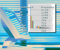
Figure 3 shows a bar chart of the first two columns of
Table 3 using Microsoft Excel 2004 for Mac. Again, the "TOTAL
(Top-50)" and "TOTAL" rows were not included.
Figure 4 shows a box plot for the Frequency column of
Table 3 again made with R using the boxplot(Frequency) command. Before
running this command, you must give attach(DATA) in order to create
separate data sets using the columns of the "DATA" data set.
The big advantage of box plots is that they are compact in size. On the
right of the box plot is a brief description of its meaning. The following
two definitions are useful:
- Percentile: We can find out 99 values
that divide our data set into 100 equal subsets. Each one of those 99
values is called a percentile.
- Outlier: An outlier is a data value that
is very big or very small with respect to the other values of a data set.
In network intrusion detection, the purpose is to find outliers (unusual
events) among a large number of regular events.
Figure 5 shows a 3-D pie chart of Table 4. It is
interesting that most of the commands are in the boundary classes (classes
1 and 5). People either use small commands or big commands.
Conclusions
So, after having all these charts and plots and boxes,
what useful conclusions and information can you get? Well, this depends on
your needs. You can use the information in many ways, including the
following:
- Depending on the number of history file
entries that you can get, you can keep weekly or monthly graphs for
comparison. Radical changes may be a sign of abnormality.
- You can find unusual commands so that you
can mine security incidents.
- If you find that most of the people are
using heavy applications, you can upgrade your system.
- You can advise people to use aliases for
the big length commands. Please note that your users may not like your
reading their commands for reasons of privacy, so advise them in a proper
way.
Being able to visualize this information makes your
life as a systems administrator easier, and sometimes it makes your
cooperation with your boss easier as well. Bosses tend to understand
graphics and images better than plain-text commands. Most of all, graphs
and charts are a high-level tool for watching many different Unix systems
at the same time.
Summary
In this article, I have shown how to categorize
command history data located in text files according to your own criteria.
Perl, the R statistical system, and Microsoft Excel 2004 for Mac were used
in this article for creating meaningful plots, graphs, and charts. No
matter what kind of Unix system you administer, the presented techniques
can make your life easier.
Acknowledgments
I thank Agisilaos, Dimitris, Georgia (she gave me two
files!), and Nikos for giving me their .bash_history files for the purposes
of this article.
References and Links
1. Tsoukalos, Mihalis. 2005. "Using the R System for Systems Administration", Sys Admin, 14(1), 40-46.
2. R Project home page -- http://www.r-project.org/
3. Venables, W.N. and B.D. Ripley. 2002. Modern Applied Statistics with S, 4th Ed. Springer Verlag.
4. Christiansen, Tom and Nathan Torkington. 2003. Perl Cookbook, 2nd Ed. O'Reilly.
Mihalis Tsoukalos lives in Greece with his wife,
Eugenia, and works as a high school teacher. He holds a B.Sc. in
Mathematics and a M.Sc. in IT from University College London. Before
teaching, he worked as a Unix systems administrator and an Oracle DBA. He
is currently writing a book about Mac OS X Dashboard Widgets. Mihalis can
be reached at: mctsouk@sch.gr.
|