One more grain of sand dropped on top of a pile of sand will usually do nothing more than make the pile a tiny bit larger. Occasionally, though, it will set off an avalanche that radically reshapes the landscape. Observations such as this form the basis of complexity theory, which holds that small events can have unpredictable, and sometimes disproportionately large, effects -- the relevance of which will become apparent momentarily.
Nearly five years ago Mike Sartain and I had just put the wraps on our x86 software renderer, Pixomatic. We had done everything we could think of to speed it up, and while it had certainly gotten a lot faster, it was still so much slower than hardware that we knew we could never close the gap. As we were setting up in the RAD Game Tools booth at Game Developers Conference one morning, I said to Mike: "Man, if only Intel had a lerp [linear interpolation] instruction!"
Mike pointed across the aisle at the Intel booth. "Maybe you should ask for one."
The odds seemed long, to say the least, but I didn't have any better ideas, so I went over and talked with Dean Macri, our developer rep. That resulted in a couple of maverick Intel architects, Doug Carmean and Eric Sprangle, coming over to chat with us later; and somehow, over the course of five years, that simple question led to a team at RAD -- which grew to include Tom Forsyth and Atman Binstock -- working with Intel to help design an instruction set extension and write a software graphics pipeline for it.
Which brings us to the present day, when at long last I get to tell you about a fascinating, and very different, extension to the x86 instruction set called Larrabee New Instructions (LRBni) -- and if that's not a perfect example of complexity theory in action, I don't know what is.
More recently, Intel has also been applying additional transistors in a different way -- by adding more cores. This approach has the great advantage that, given software that can parallelize across many such cores, performance can scale nearly linearly as more and more cores get packed onto chips in the future.
Larrabee takes this approach to its logical conclusion, with lots of power-efficient in-order cores clocked at the power/performance sweet spot. Furthermore, these cores are optimized for running not single-threaded scalar code, but rather multiple threads of streaming vector code, with both the threads and the vector units further extending the benefits of parallelization. All this enables Larrabee to get as much work out of each watt and each square millimeter as possible, and to scale well far into the future.
Larrabee is an architecture, rather than a product, with three distinct aspects -- many cores, many threads, and a new vector instruction set -- that boost performance. This architecture will first be used in GPUs, and could be used in CPUs as well.
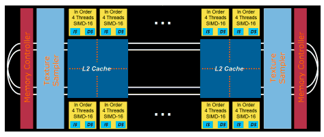
At the highest level, the architecture consists of many in-order cores, each with its own L1 and L2 cache, all sitting on a coherent interconnect bus -- which you can think of as a ring, although in fact the topology is considerably more complicated than that -- as in Figure 1.
The cores are x86 cores enhanced with vector capability, and the memory system is fully coherent. In short, Larrabee is an enhanced x86 architecture; it supports all the familiar general-purpose programming techniques and tools used on CPUs for decades, and is much like programming a lot of Core i7 cores at once. Because initial configurations are designed for use as GPUs, they lack chipset features needed to serve as a main CPU running, say, Windows; nonetheless, they are fully capable of running operating systems and general applications. For example, Larrabee, running as a GPU device under Windows, can bring up a BSD OS, with the Larrabee graphics pipeline running as just another BSD application.
Furthermore, each of those Larrabee cores supports multiple hardware threads per core (currently four, although that may change in the future). This is an important part of getting good performance out of the in-order cores; if one thread misses the cache, the other threads can keep the core busy. Threading also helps work around pipeline latency. In effect, threaded in-order cores shift the burden of extracting parallelization and working around pipeline bubbles from instruction reordering hardware to the programmer and the compiler. Without a doubt, that makes life more challenging for programmers, but the rewards are potentially large, thanks to the out-of-order hardware and associated power that can be saved.
Besides, if a program can be successfully parallelized across all those Larrabee cores, it shouldn't in principle be any more difficult to parallelize it across the threads as well. However, while this is true to a considerable extent, in actual practice issues arise because there is only one set of most core resources -- most notably caches and TLBs -- so the more threads there are performing independent tasks on a core, the more performance can suffer due to cache and TLB pressure. The graphics pipeline code on Larrabee works around this by having all the threads on each core work on the same task, using mostly shared data and code; in general, this is a fertile area for future software architecture research.
So Larrabee has lots of cores, each with multiple threads, allowing software to readily take advantage of thread-level parallelism. That's obviously critical to getting a big performance boost -- lots of cores running at high utilization are going to be much faster than even the fastest single core -- and multithreaded programming is an essential, fascinating, and challenging aspect of Larrabee. However, it's also a relatively familiar challenge from existing multicore systems, albeit taken to a new level with Larrabee, so I'm going to leave further discussion of multicore/multithreaded Larrabee programming for another day. What I'm going to delve into for the rest of this article is the third aspect of Larrabee performance -- the 16-wide vector unit, and LRBni, the instruction set extension that supports it. Together, these are designed to let software extract maximum performance from data-level parallelism -- that is, vector processing.
This is all somewhat abstract, so to make things a little more concrete, let me mention something I know for sure LRBni can do, because I've done it: software rendering with GPU-class efficiency, without any fixed-function hardware other than a texture sampler. It should be clear upon a little reflection that with a 16-wide vector unit, you can run a pixel shader on 16 pixels at a time, with the nth element of each vector instruction operating on the nth pixel of a 16-pixel block; Kayvon Fatahalian's presentation From Shader Code to a Teraflop: How Shader Cores Work discusses how this works in some detail. Somewhat less obvious is that it is possible to use LRBni to implement an efficient software rasterizer, using vector instructions to determine a triangle's pixel coverage for 16 pixels at a time.
Unfortunately, those topics are far too complex to discuss here. However, LRBni-based implementations of both rasterization and shaders will be discussed in detail in future articles.
LRBni adds two sorts of registers to the x86 architectural state. There are 32 new 512-bit vector registers, v0-v31, and 8 new 16-bit vector mask registers, k0-k7. While some core resources such as caches are shared by the core threads, that is not the case for registers; each thread has a full complement of vector and vector mask registers.
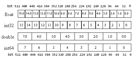
LRBni vector instructions are either 16-wide or 8-wide, so a vector register can be operated on by a single LRBni instruction as 16 float32s, 16 int32s, 8 float64s, or 8 int64s, as in Figure 2, with all elements operated on in parallel. LRBni vector instructions are also ternary; that is, they involve three vector registers, of which typically two are inputs and the third the output. This eliminates the need for most move instructions; such instructions are not a significant burden on out-of-order cores, which can schedule them in parallel with other work, but they would slow Larrabee's in-order pipeline considerably.
I discuss each of these in turn, referring to Table 1, which lists a broad sample of LRBni instructions. (Table 1 is not a complete listing; some instructions are still evolving, and others would require too much explanation.) Vector instructions start with v, and vector mask instructions start with k. The mnemonic suffixes follow the SSE convention of "px," where p means "packed" (that is, a vector of 8 or 16 elements), and x refers to the element type:
You can find additional information about LRBni, including instruction descriptions and prototyping libraries, here.
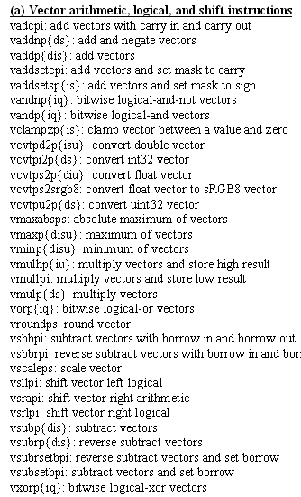
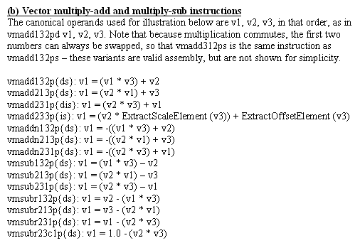
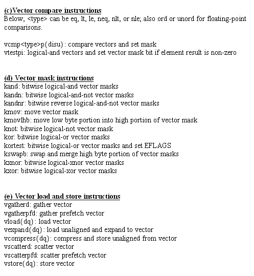
Table 1: Broad sampling of LRBni instructions.
Vector Arithmetic, Logical, and Shift Instructions
The arithmetic, logical, and shift vector instructions include everything you'd expect: add, subtract, add with carry, subtract with borrow, multiply, round, clamp, max, min, absolute max, logical-or, logical-and, logical-xor, logical-shift and arithmetic-shift by a per-element variable number of bits, and conversions among floats, doubles, and signed and unsigned int32s. There are also multiply-add and multiply-sub instructions, which run at the same speed as other vector instructions, thereby doubling Larrabee's peak flops. Finally, there is hardware support for transcendentals and higher math functions. The arithmetic vector instructions operate in parallel on 16 floats or int32s, or 8 doubles, although this is not fully orthogonal; most float multiply-add instructions have no int32 equivalent, for example. The logical vector instructions operate on 16 int32s or 8 int64s, and the shift vector instructions operate on 16 int32s only. The non-orthogonality of the vector instructions may seem a bit inconvenient, but they make for lower-power hardware, which in turn makes it possible to have more cores -- and therefore more processing power.
Both the destination and the first source operand for a vector instruction must typically be vector registers (for certain instructions, one of the first two operands must be a vector mask register, as I discuss shortly), but the last source may optionally be a memory operand; this feature comes at no performance cost and saves a great many load instructions, reducing code size and freeing up the in-order pipeline to do other work. This is the reason for the existence of the reverse-subtract instructions, and also for the many variants of multiply-add and multiply-subtract, which allow you to choose which of the three operands is added to or subtracted from, although the destination must always be a vector register. Multiply-add and multiply-sub have three vector operands like other vector instructions, but are special in that they have three sources, so the first operand must serve as both a source and the destination; hence, unlike the other instructions, most multiply-add and multiply-sub instructions have no non-destructive form. (The exception is vmadd233, a special form of multiply-add designed specifically for interpolation, which gets both offset and scale from a single operand and consequently uses only two source operands.) It's worth noting that multiply-add and multiply-sub instructions are fused; that is, no bits of floating-point precision are lost between the multiply and the add or subtract, so they are more accurate than and not exactly equivalent to a multiply instruction followed by a separate add or subtract instruction.
But wait, there's a lot more to vector instructions, which are really more like little clusters of processing functions than traditional scalar or SSE instructions -- and all at no extra cost! If there's a memory operand to a vector instruction, that operand may optionally be broadcast from one or four elements in memory up to 16 vector elements (or 8 for doubles or int64s) prior to the instruction's operation, as in Figure 3.
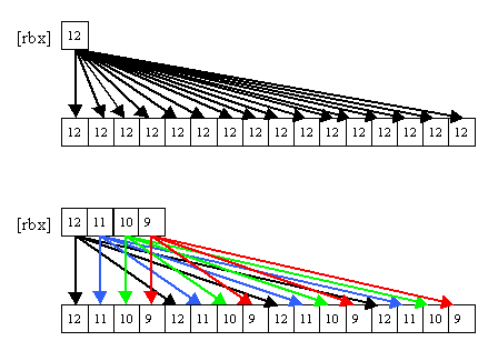
Figure 3: 1-to-16 {1to16} and 4-to-16 {4to16} broadcasts.
This is useful for keeping memory and cache footprint down when applying a scalar or a four-element vector across a vector operation. Alternatively, the source memory operand may be converted from one of several compact types (including float16) to float, or from a smaller integer to int32, as listed in Table 2. This is not only useful for keeping footprint down but also removes the need for a separate instruction to perform the conversion. However, a single instance of a load-op instruction can either convert or broadcast, but can't do both. If there is no memory operand, the last vector register operand may be swizzled in one of seven ways, as in Table 3, including one that supports efficient calculation of four cross-products at once. All load-op broadcasts, conversions, and swizzles are free, occurring during the normal course of vector instruction execution.
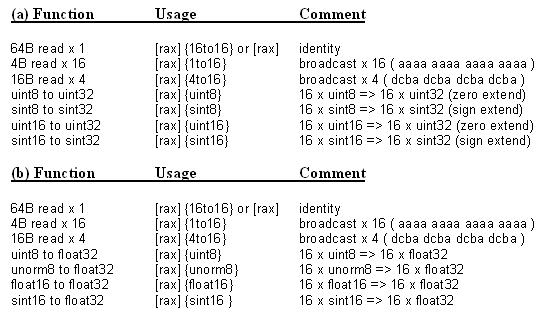
Table 2: (a) Load-op broadcasts and up-conversions for int32 operations. (b) Load-op broadcasts and up-conversions for float operations.
We're still not quite done, because every vector instruction can also perform predication. Each vector mask register contains 16 bits, neatly matching the 16 elements in a vector register. Every vector instruction can take a vector mask register as the writemask operand, and if any bit in that vector mask register is zero, the corresponding element of the destination register is left unchanged. Once again, there is no cost for this. Vector instructions can also specify no writemask, for the common case in which all 16 elements should be updated.
Table 3: Vector operand swizzles. Notation: dcba denotes the 32-bit elements
that form one 128-bit block in the source (with 'a' least-significant and 'd' most-significant), so aaaa means that the least-significant element of the 128-bit block in the source is replicated to all four elements of the same 128-bit block in the destination; the depicted pattern is then repeated for all four 128-bit blocks in the source and destination. These can be used only if there is no memory operand, and on only one operand per vector instruction. 64-bit elements are handled identically, except that in that case the above table describes 256-bit blocks, and the action is repeated for the two 256-bit blocks in the vector.
Predication makes it possible to handle the partial vector iteration at the end of vectorized loops. More importantly, it makes it possible to handle conditionals and loops in vector code.
Let's take a look at some of these features in action. First, here's a simple floating-point vector multiply:
'vmulps v0, v5, v6 ; v0 = v5 * v6
Figure 4 shows how this performs 16 multiplies in parallel.
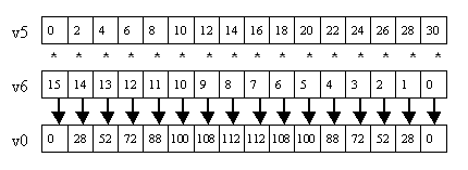
Figure 4: vmulps v0, v5, v6.
Next, let's make it a multiply-add (Figure 5):
vmadd231ps v0, v5, v6 ; v0 = v5 * v6 + v0
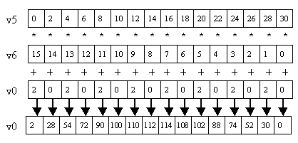
Figure 5: vmadd231ps v0, v5, v6.
Here, the destination is also the third source. In the instruction mnemonic, "231" refers to the placement of the three operands in the multiply-add equation. Thus, "madd231" means "multiply operand_2 with operand_3, add operand_1"; "madd132" would mean "multiply operand_1 with operand_3, add operand_2," which translates to "v0 = v0 * v6 + v5" for the three operands used above.
Now we'll add predication; k1 writemasks the updating of the elements (Figure 6):
vmadd231ps v0 {k1}, v5, v6
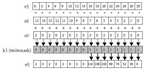
Figure 6: vmadd231ps v0 {k1}, v5, v6.
We can make one source a load-op memory operand using the standard assortment of x86 addressing modes (Figure 7):
vmadd231ps v0 {k1}, v5, [rbx+rcx*4]
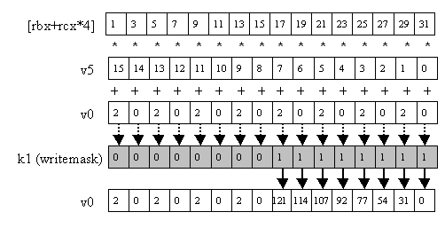
Figure 7: vmadd231ps v0 {k1}, v5, v6.
We can broadcast from 4 elements in memory to 16 elements to operate on (Figure 8):
vmadd231ps v0 {k1}, v5, [rbx+rcx*4] {4to16}
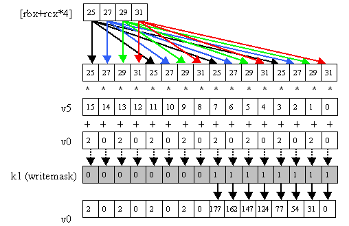
Figure 8: vmadd231ps v0 {k1}, v5, [rbx+rcx*4] {4to16}.
Or we can upconvert from float16 format (Figure 9):
vmadd231ps v0 {k1}, v5, [rbx+rcx*4] {float16}
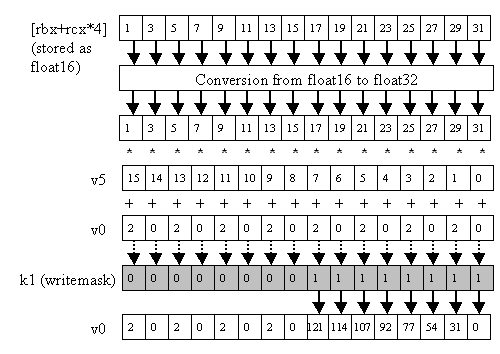
Figure 9: vmadd231ps v0 {k1}, v5, [rbx+rcx*4] {float16}.
One note here: Memory operands to vector instructions must be aligned to the size of the block of data loaded; for this purpose, it is the size before writemasking is applied that matters. Thus, the example in Figure 7 must be 64-byte aligned, but the example in Figure 8 only has to be 16-byte aligned, and the example in Figure 9 only has to be 32-byte aligned. (The alignment requirement is implementation-dependent, and could change in the future, but it will be true of the initial versions of Larrabee, at least.)
No, it's not like any x86 assembly syntax you've ever seen, but it's actually pretty straightforward, and, as you can see, for once things are spelled out pretty clearly -- "{float16}" is a lot easier to parse than most assembly-language mnemonics I've encountered.
All of the above instructions run at the same throughput (although again that's implementation dependent), and all of the capabilities illustrated above work with any vector instruction.
More About Vector Masks
Now that we've seen how predication works, let's look at how vector masks get set. They are primarily either generated by vector compares or copied from general-purpose registers (general-purpose registers are the familiar x86 scalar registers -- rax, ecx, and so on), although they can also come from add-and-generate-carry and subtract-and-generate-borrow instructions, or from a couple of special add-and-set-vector-mask-to-sign instructions designed for rasterization. Vector mask registers can also be operated on by a set of vector mask instructions. I discuss each of the primary ways of modifying vector masks next.
Vector compares have the base mnemonic vcmp, and operate as you'd imagine; the elements of one vector are compared pairwise with the elements of another vector, and the bit in the destination vector mask register that corresponds to each pair is set to the result of the comparison. The standard float, double, and signed and unsigned int32 comparisons are supported. There is also a vector test instruction, vtest, which operates similarly to vector comparison.
One interesting point is that although the vector compare instructions take a mask input, it does not operate as a normal writemask, although the operation is similar enough so that the usual writemask notation is used. With normal writemasks, 0-bits block updating of destination elements; for vector compare instructions (and vtest as well), 0-bits in the source mask result in corresponding 0-bits in the destination mask - that is, the comparison result is logical-anded with the source mask. This variant form of masking is desirable because the result will typically be used as a writemask, rather than the normal case where the result is used with a separate writemask that keeps the masked elements inactive.
This is illustrated in Figure 10 for the vector-compare-less-than-packed-single instruction:
vcmpltps k3 {k1}, v0, v2
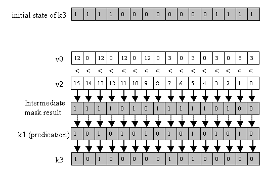
Figure 10: vcmpltps k3 {k1}, v0, v2. The initial state of the destination vector mask register is ignored; 0-bits in the source mask result in 0-bits in the destination mask
Data may also be copied between two vector mask registers, or between a vector mask register and a general-purpose register, as, for example, with:
kmov k2, eax ; k2 = ax
There are also binary instructions to perform a variety of logical operations on vector mask registers, such as:
kand k1, k0 ; k1 = k1 & k0
Finally, there is exactly one way to use the vector mask registers to set the general processor flags: with the kortest instruction. In fact, this is the only vector-related instruction of any sort that can affect the flags. Kortest logical-ors two vector mask registers together and sets the zero and carry flags based on the result; if the result is all-zeroes, ZF is set, and if the result is all-ones, CF is set, as in Figure 11.
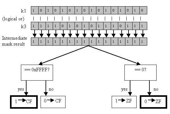
Figure 11: kortest k1, k3
Vector Loads, Stores, and Conversions
Larrabee provides both aligned and unaligned loads and stores. Like all vector instructions, loads can do 1-to-16 or 4-to-16 broadcasts. Unlike other vector instructions, however, they can also do simultaneous type conversions from smaller types to float or int32; in fact, they can do far more type conversions than can load-op instructions, supporting all common DirectX/OpenGL types, as in Table 4.
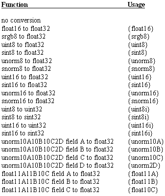
Table 4: Load conversions supported by vloadd, vexpandd, and gatherd..
Vector stores can write all 16 elements, the low four elements, or only the low element of a vector. At the same time, stores can also down-convert to the types that loads can up-convert from, with a few graphics-specific exceptions, such as sRGB, that require a separate conversion instruction (Table 5).
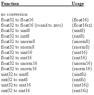
Table 5: Store conversions supported by vstored, vcompressd, and scattered.
A writemask can provide predication for vector loads and stores just as it does for other vector instructions. Once again, writemasking, broadcasting, conversion, and selection are free.
Getting Data Into and Out of Vector Format
The instructions covered so far are the heart of Larrabee's data-crunching capabilities, but by themselves they'd require all their input and output to be arranged in structure-of-arrays (SOA) form, which would be unfortunate because most data is in array-of-structures (AOS) form -- not least a lot of graphics data, such as vertex arrays. Since Larrabee's initial use will be as the processor for a graphics card, it's obviously essential to be able to get data into and out of SOA format efficiently, and LRBni adds three sorts of instructions for this purpose. Of these, first and most important are the gather/scatter instructions.
The key to gather is that it lets you load each element of the destination vector from any memory address, independent of where the other elements are being loaded from, as in Figure 12, which I'll discuss shortly. If you think of this as performing a separate scalar load for each element, it's obvious why it's so useful for vectorization -- it's the vector load instruction for cases where each of the 16 streams has a different data source.
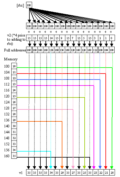
Figure 12: vgatherd v1 {k1}, [rbx + v2*4]. This is a simplified representation of what is currently a hardware-assisted multi-instruction sequence, but will become a single instruction in the future.
Consider the case of checksumming an int32 array. If it's just one array, you can process it 16 values at a time, using the normal vector load instruction, vload, followed by vaddpi, to sum 16 values at a pop; or you could just do a load-op vadd, as in Listing One. Then, at the end, you can sum together the 16 values you've accumulated, and you're done. (If the array wasn't a multiple of 16 in length, you'd use the writemask to do a partial sum at the end.)
; Partial code to calculate an array checksum, summing

; 16 elements at a time; code after the loop to do a final

; sum of the 16 partial sums would also be required.

; On entry:

;   rbx points to the base of the array to sum.

;   rcx is how many elements to sum.

; On exit, v0 contains the 16 partial sums.

	vxorpi	 v0, v0, v0

	shr		rcx, 4	; do 16 at a time

ChecksumLoop:

	vaddpi	v0, v0, [rbx]

	add	rbx, 64

	dec	rcx

	jnz	ChecksumLoop
Listing One
If, however, the value you were checksumming was a field in a structure, so a skip was required between each addition, the vgatherd instruction would allow you to parallelize in either of two different ways. You could gather 16 fields at a time from the array, as in Listing Two.
; Partial code to calculate the checksum of a specific field in

; an array of structures, summing 16 elements at a time; code

; after the loop to do a final sum of the 16 partial sums would

; also be required.

; On entry:

;   v2 contains the offsets of the first 16 checksum fields

;        in the array relative to rbx.

;   rcx is how many elements to sum.

; On exit, v0 contains the 16 partial sums.

	vxorpi		v0, v0, v0

	shr		rcx, 4	; do 16 at a time

ChecksumLoop:

	vgatherd	v1 {k0}, [rbx + v2]

	vaddpi		v0, v0, v1

	; step to the next 16 values to checksum

	vaddpi		v2, v2, [Mem_Structure_Size_Times_16] {1to16}

	dec		rcx

	jnz		ChecksumLoop
Listing Two
Or, more generally, you could process 16 different streams and do 16 sums at once, one from each of 16 different arrays; you'd gather 16 values, one from each array, and then vaddpi them, as in Listing Three. When ChecksumLoop in Listing 3 finishes, you will have accumulated the 16 sums for the 16 arrays. The structure size can even be different for each array. (Note that Listings Two and Three are almost identical; gather is so flexible that the same gather-based code can do many different things, depending on the initial conditions.)
; Calculates checksums of a specific field in 16 arrays of structures in parallel.

; On entry:

;   v2 contains the 16 offsets of the checksum field in each of the

;        16 arrays relative to rbx.

;   rcx is how many elements to sum.

; On exit, v0 contains the 16 checksums.

	vxorpi		v0, v0, v0

ChecksumLoop:

	vgatherd	v1 {k0}, [rbx + v2]

	vaddpi		v0, v0, v1

	; step to the next value in each array

	vaddpi		v2, v2, [Mem_Structure_Sizes]

	dec		rcx

	jnz		ChecksumLoop
Listing Three
Okay, those last two code listings require a bit of explanation, because the gather/scatter instructions do not follow normal addressing rules. The address for a gather or scatter is formed from the sum of a base register and the elements of a scaled index vector register, as in Figure 12. This is the only case in which a vector register can be used to address memory. More precisely, for each element to be loaded, the address is the sum of the base register and the sign-extension to 64 bits of the corresponding element of the index vector register, optionally scaled by 2, 4, or 8. Note that the 32-bit size of the elements used for the index results in a 4 GB limit on the range for gather/scatter (or larger if scaling by 2, 4 or 8).
What if your gather targets aren't all contained within a 4 GB range? Then you need to wrap another loop around the basic gather loop, in order to step through the 4 GB ranges touched by the gather addresses, which is somewhat more complicated, but not unduly so.
All of the above applies for scatters, but in reverse.
Finally, gather and scatter support all the data conversions that vload and vstore, respectively, support, as well as writemasking. They don't support broadcast or store selection, since those would be useless for these instructions -- to broadcast in a gather, just set all the index fields to the same value (a partial broadcast is performed in Figure 12), and scatter can similarly easily perform store selection.
Another important feature is the ability to queue data efficiently with the vcompress and vexpand instructions. For vcompress, the writemask-enabled elements of the source vector are stored sequentially in memory, as in Figure 13; for vexpand, the writemask-enabled elements of the destination are loaded from a sequential stretch of memory, reversing the action of vcompress, as in Figure 14. A new scalar instruction, countbits, has been added so that the number of enabled bits in a vector mask register -- and thus the number of elements stored by vcompress or loaded by vexpand -- can easily be counted.
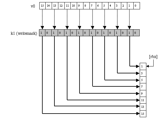
Figure 13: vgatherd v1 {k1}, [rbx + v2*4]. : vcompressd [rbx] {k1}, v0. This is a simplified representation of what is currently a two-instruction sequence.
As with all vector instructions vcompress and vexpand can be used without specifying a writemask, in which case all elements are loaded or stored, with no compression or expansion needed. In this mode, vcompress and vexpand function as unaligned store and load.
Finally, the bsf and bsr bit-scan instructions have been enhanced. Where the existing bsf instruction finds the first 1-bit starting from bit 0 and scanning up, the new bsfi instruction finds the first 1-bit starting from the bit above the bit specified by the destination operand. This allows bsfi to continue a search started with bsf, without any bit-clearing overhead. The bsri instruction similarly provides a starting point for reverse bit scans. These instructions are useful for parallel-to-serial conversion when the results of a vector operation must be processed serially, as we will see when we look at rasterization.
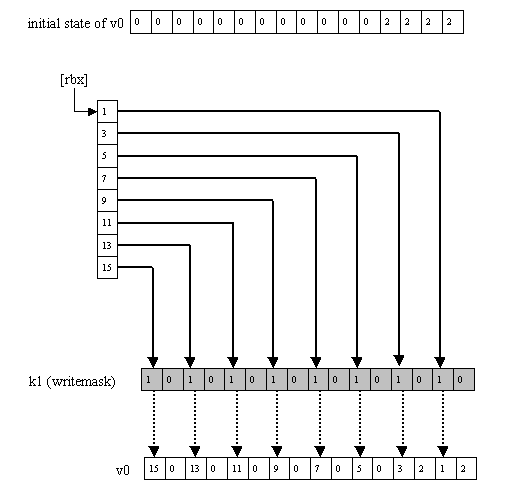
Figure 14: vexpandd v0 {k1}, [rbx]. This is a simplified representation of what is currently a two-instruction sequence.
The Rest of LRBni
Several vector instructions have been added for moving bits around within each element. Vinsertfield rotates each source element according to a per-instruction immediate value, then masks off a portion of the result according to two more immediate values, and leaves the destination element untouched where the mask is zero, effectively inserting the rotated source element into the destination element, as in Figure 15. (In this case "mask" just means a normal bitmask, of the sort you might logical-and with a register, not the writemask.) Used with no bitmask, vinsertfield can also serve as a rotate-by-immediate vector instruction.
Figure 15: vinsertfield v0, v1, 8, 4, 23 for element 0 of v0 and v1. The same rotation and masking is repeated for all 16 elements.
vbitinterleave11pi and vbitinterleave21pi allow the interleaving of bits from two registers; vbitinterleave11pi alternates bits from the two sources, starting with bit 0 of the last source, and vbitinterleave21pi alternates one bit from the last source with two bits from the first source. Bit-interleaving is useful for generating swizzled addresses, particularly in conjunction with vinsertfield, for example in preparation for texture sample fetches (volume textures in the case of vbitinterleave21pi). The following sequence generates 16 offsets into a fully-swizzled 256x256 four-component float texture from 16 8-bit x coordinates stored in v1 and 16 8-bit y coordinates stored in v2, as in Figure 16:
vxorpi v3, v3, v3

vbitinterleave11pi v0, v2, v1

vinsertfield v3, v0, 4, 4, 19
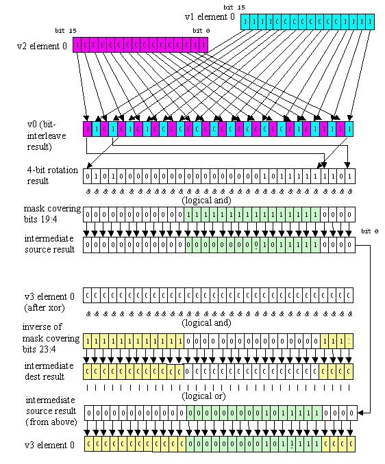
Figure 16: The operation of the instruction sequence:
vxorpi v3, v3, v3
vbitinterleave11pi v0, v2, v1
vinsertfield v3, v0, 4, 4, 19
for element 0 of v0, v1, v2, and v3. The same rotation and masking is repeated for all 16 elements. The x and y coordinates are 8-bit; the upper 8 bits of each are ignored, and in the example above are set to non-zero values in order to illustrate the masking operation of vinsertfield.
(Note that if it was a gather instruction that was going to use these indices, and if the texel size was 8 or less, it wouldn't be necessary to use vinsertfield to shift up the address in order to address the texels, since the gather instruction can scale by 2, 4, or 8.)
There are also shuffle instructions for permuting elements from a source vector to a destination vector.
Although LRBni is primarily a vector instruction extension, it adds a few scalar instructions as well. In addition to bsfi and bsri, it adds insertfield, bitinterleave11, and bitinterleave21, the scalar versions of the vector bit-manipulation instructions described above. Prefetching and other cache-control instructions have been added as well; these are particularly important on Larrabee, where data must be fetched far enough ahead and at a high enough rate to keep the voracious vector units well-fed and fully loaded in streaming applications, without the help of out-of-order hardware.
Finally, note that in the initial version of the hardware, a few aspects of the Larrabee architecture -- in particular vcompress, vexpand, vgather, vscatter, and transcendentals and other higher math functions -- are implemented as pseudo-instructions, using hardware-assisted instruction sequences, although this will change in the future.
What Does It All Add Up To?
I'd sum up my experience in writing a software graphics pipeline for Larrabee by saying that Larrabee's vector unit supports extremely high theoretical processing rates, and LRBni makes it possible to extract a large fraction of that potential in real-world code. For example, real pixel-shader code running on simulated Larrabee hardware is getting 80% of theoretical maximum performance, even after accounting for work wasted by pixels that are off the triangle but still get processed due to the use of 16-wide vector blocks.
Tim Sweeney, of Epic Games -- who provided a great deal of input into the design of LRBni -- sums up the big picture a little more eloquently:
Larrabee enables GPU-class performance on a fully general x86 CPU; most importantly, it does so in a way that is useful for a broad spectrum of applications and that is easy for developers to use. The key is that Larrabee instructions are "vector-complete."
More precisely: Any loop written in a traditional programming language can be vectorized, to execute 16 iterations of the loop in parallel on Larrabee vector units, provided the loop body meets the following criteria:
- Its call graph is statically known.
- There are no data dependencies between iterations.
Shading languages like HLSL are constrained so developers can only write code meeting those criteria, guaranteeing a GPU can always shade multiple pixels in parallel. But vectorization is a much more general technology, applicable to any such loops written in any language.
This works on Larrabee because every traditional programming element -- arithmetic, loops, function calls, memory reads, memory writes -- has a corresponding translation to Larrabee vector instructions running it on 16 data elements simultaneously. You have: integer and floating point vector arithmetic; scatter/gather for vectorized memory operations; and comparison, masking, and merging instructions for conditionals.
This wasn't the case with MMX, SSE and Altivec. They supported vector arithmetic, but could only read and write data from contiguous locations in memory, rather than random-access as Larrabee. So SSE was only useful for operations on data that was naturally vector-like: RGBA colors, XYZW coordinates in 3D graphics, and so on. The Larrabee instructions are suitable for vectorizing any code meeting the conditions above, even when the code was not written to operate on vector-like quantities. It can benefit every type of application!
A vital component of this is Intel's vectorizing C++ compiler. Developers hate having to write assembly language code, and even dislike writing C++ code using SSE intrinsics, because the programming style is awkward and time-consuming. Few developers can dedicate resources to doing that, whereas Larrabee is easy; the vectorization process can be made automatic and compatible with existing code.
In short, it will be possible to get major speedups from LRBni without heroic programming, and that surely is A Good Thing. Of course, nothing's ever that easy; as with any new technology, only time will tell exactly how well automatic vectorization will work, and at the least it will take time for the tools to come fully up to speed. Regardless, it will equally surely be possible to get even greater speedups by getting your hands dirty with intrinsics and assembly language; besides, I happen to like heroic coding. So in the next article we'll look under the hood, examining how rasterization, a process that is most definitely not inherently parallel, can be efficiently implemented with LRBni.