Thomas E. Janzen was born in Chicago and raised in Seattle and Los Angeles. A musician and performance artist, he has published in computer music, particularly about his improvising program, AlgoRhythms. As a software engineer, he has developed software to test integrated circuits, to test newly manufactured workstations, and to analyze measurements. He is currently unemployed in Hudson, Massachusetts, and can be reach by email at tej@world.std.com.
Introduction
When you look at something, it moves. When you try to measure a quantity, it changes. When you measure the rise time of a step function through a network of microwave switches and semi-rigid cables, it is corrupted by the network, cables, and even by the oscilloscope used to sample the waveform. Removing the corruption introduced by experimental set-ups is an old problem. Many rules-of-thumb have been recommended to reconstruct data as it is before it enters measurement equipment. Some that I have used include:
- averaging many samples of the same event
- smoothing the data with filters
- using simple arithmetic corrections
The relationship between an original signal, the impulse response of an electrical or acoustical network, and the output of the network can be expressed with the operation known as convolution. If the output and impulse response are known, then the inverse operation, deconvolution, can recover an approximation of the original input. I present here an implementation in C of an approach to direct deconvolution.
Convolution
Convolution is a widely useful function. In one dimension, it can express the relationship between the sound heard by the violinist and that heard in the last row of the balcony. It can also express the way an electrical signal is altered by passive networks and cables. Convolution can be used in digital signal processing to create finite-impulse-response filters. Convolution is the basis of important theorems in statistics and Fourier analysis.In two dimensions, convolution can be applied to anti-aliasing functions in graphics, or the response of an optical system. I will restrict myself to convolution in the time domain in one dimension. My experience is in transmission line corruption of electrical signals.
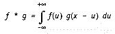
Convolution in the continuous, real domain is defined as follows:
Convolution follows the associative, commutative, and distributive laws:
- Associative:
(f * g) * h = f * (g * h)
f * g = g * f
a (f * g) = (af * ag)Here, a is a constant, f and g are functions.
The theorem in statistics is as follows:
If two independent random variables, X and Y, have a joint density function f(x,y), the density function of U = X + Y is X * Y.
The theorem in Fourier analysis can be written, using F as the Fourier operation:
F{f * g} = F{f} * F{g}
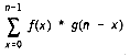
In the continuous domain, convolution operates on functions. But in practical engineering, discrete data is the rule. Such digitally-sampled waveforms might be downloaded from oscilloscopes or read from audio samplers in the backplane of your computer. In the discrete domain, the integral becomes a summation:
The arrays f and g should begin with zeros, by nature. If the function is truncated to meet this requirement, errors will be produced. If the truncation causes a small step, the errors may be small. If it causes a large step, the errors will be severe.
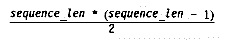
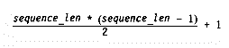
Convolution is not difficult to express in C with arrays and for loops. Listing 1 shows a function that convolves two arrays, f and g, and puts the result in array y. Note that you must provide sufficient storage for all three, defined by sequence_len times the size of a double on your system. Because convolution follows the commutative law, it doesn't matter how you arrange the two known functions in the arguments f and g. The array arguments f and g, and the length sequence_len are declared const because the convolution function does not change them.
The number of multiplications performed by this function is:
Although it is true that the commutative law allows us to treat the two convolving functions interchangeably, in practice they usually have an asymmetrical relationship. One of the functions under the summation is a stimulus to a system (such as a cap gun firing in a theater) and the other function under the summation is the unit impulse response of the system (the shot and its reverberation heard from a particular seat in the theater).
Once the impulse response is known, it can be used on other signals (such as a synthesized violin sound) to emulate the response of the system (giving the sound of playing a synthesized violin in the hall, without actually going there). In this case, the cap gun shot was also a suitable impulse for directly measuring a concert hall. When a new stimulus is convolved with the impulse response of the system, we get the simulated response of the system to that new stimulus.
Deconvolution
Under some circumstances, the result of convolution is known, while one of the convolving functions is unknown (f or g above). In order to find the unknown function, it is necessary to invert the convolution function. This new function is called deconvolution. It is described in a paper by N.S. Nahman (1986). The expression for deconvolution in the discrete domain is:
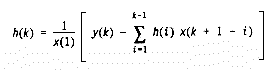
This is implemented in C in Listing 2. Although the result is called h as if it were an impulse response, this function can be called to find either function under the convolution summation, whether it is an impulse response, or a stimulus function.
The number of multiplications performed by this function can be found from:
The following restrictions appear to hold in order for this approach to direct deconvolution to work:
1. The two functions, one the result of convolution and the other one of the functions under the summation, should both begin with zero.
2. The known function from under the summation must have a non-zero value in element [1]. Otherwise the division will overflow.
3. The impulse response, known or not, must have an area between -1 and +1. Otherwise the system response is not passive, because it is amplifying the input. The described technique does not converge if this is so. You can measure the area of the impulse response if it is the known function under the summation by adding all of the elements in the array. If the system response is unknown and has an area greater than one, the given technique will not give a good answer.
4. The sequences must really be "consistent," that is, related by a system response that is passive and without feedback. Otherwise this technique will not return a useful answer.
5. The response must be later in time (in higher array positions) than then either the impulse response or the input. This is part of being consistent. Note that the impulse response includes time delay in the system that is being stimulated. You are free to experiment with shifting the impulse response back and forth within the array that holds it, to simulate different delays.
6. The impulse response, whether known or not, must be truncated (finite); zero should appear in the first and last array elements. This introduces errors, but the errors may be tolerable if the truncated function is close to the original function.
7. The members of the array of the known function under the summation should be between -1 and +1. You are free to scale all values in the stimulus and response in such a way as to make the response magnitude smaller in value than that of the stimulus, and then re-scale them to true values later.
8. If either function is at all noisy, deconvolution may not give a useful answer. This is true for two reasons:
- Noise injected separately into the output is not consistent with (the result of) any event on the input.
- The output is not consistent with noise introduced on the input after the input was introduced to the network under test.
- Average several samples of the same repeating event.
- Filter in the time domain. For example, convolve the data with a rectangular pulse with unit area. The function at the top of Figure 1 was synthesized using fun_step in Listing 3. Noise was added using fun_noise in Listing 3. (A header for the library in Listing 3 is in Listing 4. ) A unit pulse was built by fun_unit_step in Listing 3 and convolved with the noisy function to produce the smoothed function on the bottom of Figure 1.
Applying Deconvolution
The convolution function is intended for two different situations.
Situation 1:
Known functions: The calculated or sampled system impulse response, and the sampled response to a stimulus function.Unknown function: The stimulus function.
Call:
deconvolve_wave(ary_len, system_impulse_response,
     response_to_the_stimulus, stimulus_function)
Result: In stimulus_function, the approximate, reconstructed stimulus that caused the response.
Situation 2:
Known functions: The sample of a short, wide-bandwidth event, and the sampled response to the short event.Unknown function: The system impulse response.
Call:
deconvolve_wave(ary_len, short_wide_band_event,
   response_to_the_short_event, impulse_response);
Result: In impulse_response, the estimated impulse response of the system.
My work measuring high-speed circuits required extreme accuracy. I hand-built a network of semi-rigid coaxial cables (resembling model copper pipes), microwave switches, and an oscilloscope with high-speed sampling heads. As careful as I was, this setup had reflections and discontinuities that corrupted the signal, but in a passive way. The resulting signal was still fairly clean, but did have small bumps and valleys in it on the scope face. In addition, the high-frequency components were slightly attenuated. I needed the switches and cables to automate the selection of signals for measurement under the control of a microcomputer; manual cable-moving was much too slow. In order to correct for corruptions, I deconvolved the sampled waveform against the known impulse response of the system in order to recover the signal as it was before entering the matrix.
First, I measured the step response of the system. (See Figure 3. ) Stimulating the matrix with a high-performance step generator, I used the scope to sample the step twice. First, I bypassed the cable network, and directly connected the step generator to the scope using a special higher-performance head that was unsuitable for day-to-day use (the top of Figure 3) . Second, I connected the step generator to the cables and switch matrix used for measurements, and used the usual sampling head (bottom of Figure 3) . This gave me:
- the step function straight from the generator
- the step response of the cables and the usual sampling head
When sampling a test circuit through the network using the usual (lower-bandwidth) sampling head, I could deconvolve the sampled waveform against the calculated impulse response to find an approximation of the signal as it was before it entered the switching matrix and sampling head.
Figure 2 shows four waveforms. The top waveform is a step synthesized by fun_step_real in Listing 3, and is typical of some high-speed circuits. Below the step is an ideal impulse response synthesized by fun_unit_gauss_dens in Listing 3. These two functions were convolved with the function in Listing 1 to produce the third waveform, which is slightly smoothed and delayed by the impulse response. The fourth waveform is a reconstructed impulse response by calling deconvolve_wave in Listing 2 as follows:
deconvolve_wave(array_length,
             step_on_top,
             third_waveform,
             reconstructed_-
             response);
This reconstructed response is somewhat noisy, even when ideal data arrays were used. This may be due to the truncation (zeroed first member) of the impulse response and input waveform.
Calculating Risetimes
As stated above in the section on convolution, a joint density function of two gaussian density distributions is also gaussian, and its standard deviation is the root of the sum of the squares of the standard deviations of the original independent random variables.

This is true of any interval along the horizontal axis measured between the same vertical values (probabilities). This is also true if the functions are inverted (1 - ). The rising edge of some pulse circuits closely resembles one side of an inverted gaussian density distribution (synthesized by fun_step_real in Listing 3) .
The impulse response of many high-performance pulse measurement systems are also close to gaussian density distributions. This approximation can be exploited for correcting the measurements of pulse edge times (for example, the time it took an edge to move from 20% full value to 80% full value). The output edge time may be said to be the root of the sum of the squares of the system rise time and the input rise time.

(See Figure 4. )
However, as demands for accuracy and bandwidth increase, this approximation weakens. Deconvolution can make a better approximation.
Conclusion
The technique presented here for direct deconvolution is an approximation with many restrictions. Nevertheless, it is very useful both for characterizing the impulse response of a passive system and for recovering stimulus functions prior to corruptions introduced by a wide variety of networks — electrical, acoustic, and mechanical. It could even be used to decompose a statistical density function from a joint density function, although it is typically not necessary to call on such unusual techniques to do so.The presentation here was simplified. For a more sophisticated and general approach, see N.S. Nahman's paper in the References below. Although I did not incorporate deconvolution into my test process, my attempts with it were very promising, and you may find it so as well.
Government Publications
I first read about deconvolution in a paper from the National Institute of Standards and Technology. To order papers or a catalog from the NIST, contact the General Services Administration in your area, or the Government Printing Office at
Superintendent of Documents
U.S. Government Printing Office
Washington, DC 20402
(202)783-3238
NTIS may be contacted at:
National Technical Information Service
5285 Port Royal Road
Springfield, VA 22161
Your local Department of Commerce District Office may have some NIST publications.
Dr. Nahman's paper (below) is now available from
Kluwer Academic Publishers
190 Old Derby St.
Hingham, MA 02043
References
Blood, William R. 1983. MECL System Design Handbook. Motorola.Foley, James D.; van Dam, Andries; Feiner, Steven K.; Hughes, John F. 1990. Computer Graphics Principles and Practice. Addison-Wesley Publishing Company. Reading.
Lovrich, Al; Simar, Ray Jr. 1986. "Implementation of FIR/IIR Filters with the TMS32010/TMS32020," Digital Signal Processing Applications with the TMS320 Family. Texas Instruments.
Nahman, N.S. 1986. Software Correction of Measured Pulse Data. In Fast Electrical and Optical Measurements, eds. J.E. Thompson and L.H. Luessen, pp. 351-417. NATO Advanced Studies Institute Series E, no. 108. Dordrect; Netherlands: Martinus Nijhoss Publishers.
Spiegel, Murray R. 1974. Fourier Analysis with Applications to Boundary Value Problems. McGraw-Hill: New York.
Spiegel, Murray R. 1975. Probability and Statistics. McGraw-Hill: New York.
(C) 1993 Thomas E. Janzen.